Basic Signal Filters

This post contains interactive components (experimental) that allows you to execute RAVE code from the web browsers. If you would like to try this feature and customize/play with the code, please be patient. It might take a while for the browser to finish setting up (depending on your network speed). Once the script is ready, you will see “WEBR STATUS: 🟢 Ready!” in the above banner.

1. Preparation

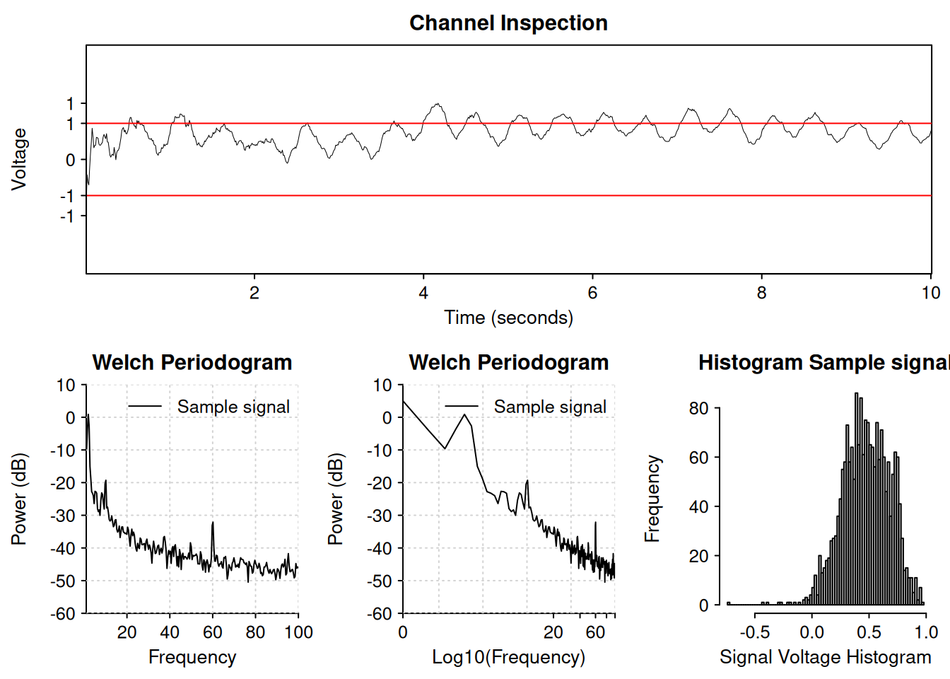
Let’s load the package and generate a sample signal. The signal is a mixture of 2Hz, 10Hz, 60Hz, and noise

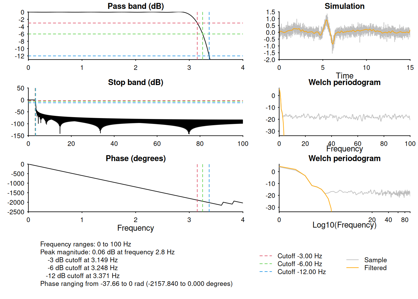
2. FIR Filter

Construct a FIR filter with low pass at 3Hz and (around) 0.5Hz transition bandwidth:

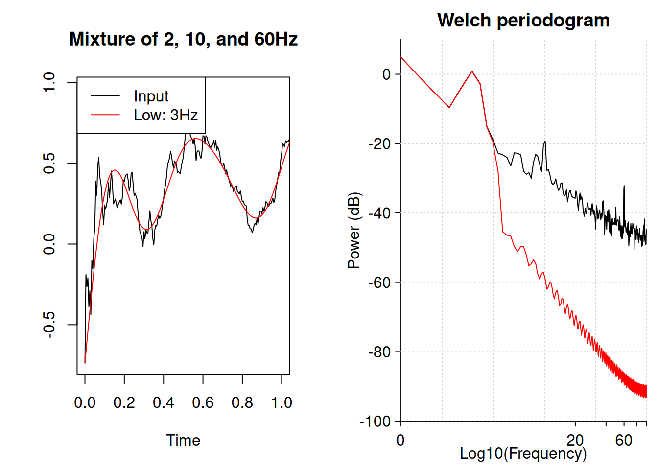
Apply the filter to the signal x using filtfilt method: